
Analyzing results#
Optimas provides a convenient ExplorationDiagnostics
class to easily analyze and visualize the output of an exploration without
having to manually access each file.
The examples below showcase the functionality of this class by analyzing the output of this basic Bayesian optimization example.
Import and initialize diagnostics#
The diagnostics class only requires the path to the exploration directory as input parameter.
[2]:
from optimas.diagnostics import ExplorationDiagnostics

diags = ExplorationDiagnostics("./exploration")
[INFO 07-10 23:33:14] optimas.generators.base: Completed trial 0 with objective(s) {'f': np.float64(-83.717461)}
[INFO 07-10 23:33:14] optimas.generators.base: Completed trial 1 with objective(s) {'f': np.float64(-13.042072)}
[INFO 07-10 23:33:14] optimas.generators.base: Completed trial 2 with objective(s) {'f': np.float64(66.569828)}
[INFO 07-10 23:33:14] optimas.generators.base: Completed trial 3 with objective(s) {'f': np.float64(-111.478379)}
[INFO 07-10 23:33:14] optimas.generators.base: Completed trial 4 with objective(s) {'f': np.float64(-41.256479)}
[INFO 07-10 23:33:14] optimas.generators.base: Completed trial 5 with objective(s) {'f': np.float64(-118.854042)}
[INFO 07-10 23:33:14] optimas.generators.base: Completed trial 6 with objective(s) {'f': np.float64(-141.84533)}
[INFO 07-10 23:33:14] optimas.generators.base: Completed trial 7 with objective(s) {'f': np.float64(-9.127097)}
[INFO 07-10 23:33:14] optimas.generators.base: Completed trial 8 with objective(s) {'f': np.float64(-178.313156)}
[INFO 07-10 23:33:14] optimas.generators.base: Completed trial 9 with objective(s) {'f': np.float64(-42.156296)}
[INFO 07-10 23:33:14] optimas.generators.base: Completed trial 10 with objective(s) {'f': np.float64(-247.727993)}
[INFO 07-10 23:33:14] optimas.generators.base: Completed trial 11 with objective(s) {'f': np.float64(-101.69936)}
[INFO 07-10 23:33:14] optimas.generators.base: Completed trial 12 with objective(s) {'f': np.float64(-395.347533)}
[INFO 07-10 23:33:14] optimas.generators.base: Completed trial 13 with objective(s) {'f': np.float64(-252.64064)}
[INFO 07-10 23:33:14] optimas.generators.base: Completed trial 14 with objective(s) {'f': np.float64(-292.85467)}
Access exploration history#
The diagnostics provide easy access to the exploration history, which
is returned as a pandas DataFrame.
[3]:
diags.history
[3]:
| trial_index | trial_status | trial_ignored | x0 | x1 | f | cancel_requested | gen_ended_time | gen_informed | gen_informed_time | ... | given_back | kill_sent | num_gpus | num_procs | sim_ended | sim_ended_time | sim_id | sim_started | sim_started_time | sim_worker | |
|---|---|---|---|---|---|---|---|---|---|---|---|---|---|---|---|---|---|---|---|---|---|
| 0 | 0 | COMPLETED | False | 0.908175 | 11.139719 | -83.717461 | False | 1.752190e+09 | True | 1.752190e+09 | ... | False | False | 0 | 1 | True | 1.752190e+09 | 0 | True | 1.752190e+09 | 1 |
| 1 | 1 | COMPLETED | False | 14.597818 | 4.111499 | -13.042072 | False | 1.752190e+09 | True | 1.752190e+09 | ... | False | False | 0 | 1 | True | 1.752190e+09 | 1 | True | 1.752190e+09 | 2 |
| 2 | 2 | COMPLETED | False | 3.482295 | 15.000000 | 66.569828 | False | 1.752190e+09 | True | 1.752190e+09 | ... | False | False | 0 | 1 | True | 1.752190e+09 | 2 | True | 1.752190e+09 | 1 |
| 3 | 3 | COMPLETED | False | 0.000000 | 6.799421 | -111.478379 | False | 1.752190e+09 | True | 1.752190e+09 | ... | False | False | 0 | 1 | True | 1.752190e+09 | 3 | True | 1.752190e+09 | 2 |
| 4 | 4 | COMPLETED | False | 0.717630 | 0.000000 | -41.256479 | False | 1.752190e+09 | True | 1.752190e+09 | ... | False | False | 0 | 1 | True | 1.752190e+09 | 4 | True | 1.752190e+09 | 1 |
| 5 | 5 | COMPLETED | False | 0.000000 | 14.746336 | -118.854042 | False | 1.752190e+09 | True | 1.752190e+09 | ... | False | False | 0 | 1 | True | 1.752190e+09 | 5 | True | 1.752190e+09 | 2 |
| 6 | 6 | COMPLETED | False | 0.000000 | 11.550430 | -141.845330 | False | 1.752190e+09 | True | 1.752190e+09 | ... | False | False | 0 | 1 | True | 1.752190e+09 | 6 | True | 1.752190e+09 | 1 |
| 7 | 7 | COMPLETED | False | 10.032862 | 0.000000 | -9.127097 | False | 1.752190e+09 | True | 1.752190e+09 | ... | False | False | 0 | 1 | True | 1.752190e+09 | 7 | True | 1.752190e+09 | 2 |
| 8 | 8 | COMPLETED | False | 11.457939 | 15.000000 | -178.313156 | False | 1.752190e+09 | True | 1.752190e+09 | ... | False | False | 0 | 1 | True | 1.752190e+09 | 8 | True | 1.752190e+09 | 1 |
| 9 | 9 | COMPLETED | False | 8.327989 | 15.000000 | -42.156296 | False | 1.752190e+09 | True | 1.752190e+09 | ... | False | False | 0 | 1 | True | 1.752190e+09 | 9 | True | 1.752190e+09 | 2 |
| 10 | 10 | COMPLETED | False | 12.349574 | 15.000000 | -247.727993 | False | 1.752190e+09 | True | 1.752190e+09 | ... | False | False | 0 | 1 | True | 1.752190e+09 | 10 | True | 1.752190e+09 | 1 |
| 11 | 11 | COMPLETED | False | 10.820532 | 15.000000 | -101.699360 | False | 1.752190e+09 | True | 1.752190e+09 | ... | False | False | 0 | 1 | True | 1.752190e+09 | 11 | True | 1.752190e+09 | 2 |
| 12 | 12 | COMPLETED | False | 12.549258 | 12.536054 | -395.347533 | False | 1.752190e+09 | True | 1.752190e+09 | ... | False | False | 0 | 1 | True | 1.752190e+09 | 12 | True | 1.752190e+09 | 1 |
| 13 | 13 | COMPLETED | False | 12.778762 | 15.000000 | -252.640640 | False | 1.752190e+09 | True | 1.752190e+09 | ... | False | False | 0 | 1 | True | 1.752190e+09 | 13 | True | 1.752190e+09 | 2 |
| 14 | 14 | COMPLETED | False | 12.676322 | 11.326142 | -292.854670 | False | 1.752190e+09 | True | 1.752190e+09 | ... | False | False | 0 | 1 | True | 1.752190e+09 | 14 | True | 1.752190e+09 | 1 |
15 rows × 22 columns
Built-in plotting utilities#
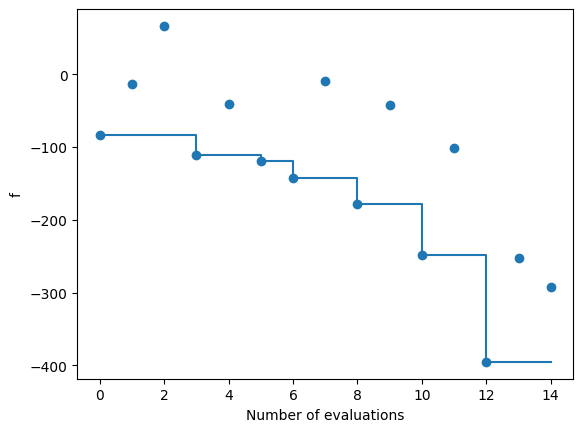
Several basic plotting functions are provided by the diagnostics class.
The example below uses
plot_objective()
to show the value of the objective f for each evaluation, as well as
the evolution of the cumulative best.
[4]:
diags.plot_objective(show_trace=True)
User plots#
The ExplorationDiagnostics exposes all
necessary data to perform any analysis or plot of the exploration.
As an example, the code below generates a plot of the phase-space of the
optimization, including the value of each evaluation and the boundaries of
the varying parameters.
[5]:
import matplotlib.pyplot as plt

fig, ax = plt.subplots()
vps = diags.varying_parameters
df = diags.history
f1 = diags.objectives[0]
ax.axvline(vps[0].lower_bound)
ax.axvline(vps[0].upper_bound)
ax.set_xlabel(vps[0].name)
ax.axhline(vps[1].lower_bound)
ax.axhline(vps[1].upper_bound)
ax.set_ylabel(vps[1].name)
ax.scatter(df[vps[0].name], df[vps[1].name], c=df[f1.name])
[5]:
<matplotlib.collections.PathCollection at 0x76f40e6608d0>
